서포트 벡터 머신이란(이하 SVM)
서포트 벡터 머신은 결정 경계(Decision Boundary), 즉 분류를 위한 일종의 기준선을 정의하는 모델.
새로운 점이 주어졌을 때 경계에 의해 분류됨
핵심은 이 결정 경계를 어떻게 정의하고 계산하는 것.
아래는 데이터의 속성(feature) 이 두개일 경우 생각해보면 결정경계는 아래 예시와 같이 일차함수로 간단히 정의됨

속성이 3개가 될 경우에는 다음과 같이 3차원 공간에서 면으로 정의됨

최적의 결정 경계는?
그럼 해결해야하는 문제는 최적의 결정 경계를 정하는 것
아래의 그래프들 중에서 무엇이 나을까 생각해보면 E랑 F랑 좀 아리송하긴 하지만 F라는 걸 알 수 있는데 이는 결정 경계가 두 클래스와 가장 멀리 떨어져 있기 때문이다.
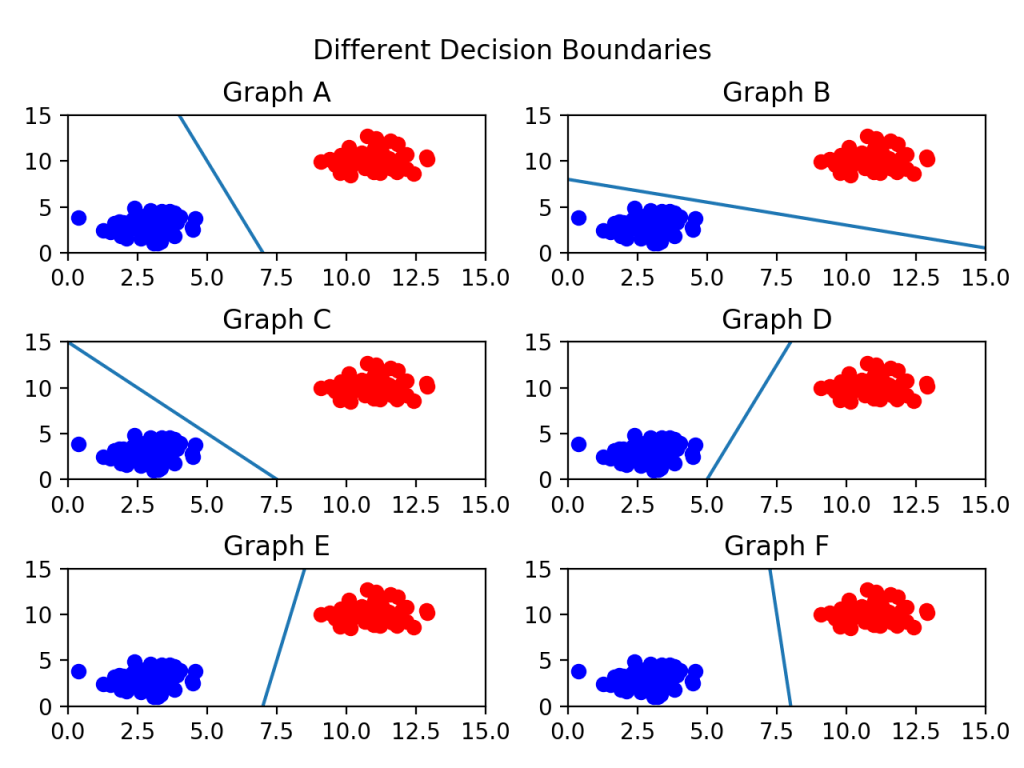
정리를 해보자면 결정경계는 데이터 군으로부터 거리가 가장 먼 게 최적이라고 할 수 있음
서포트 벡터 머신이라는 이름 자체에서 서포트 벡터는 결정 경계와 가까이 있는 데이터 포인트를 의미
즉 서포트 벡터들이 데이터들이 경계를 정의하는 결정적인 역할을 하는 것
마진(Margin)
마진은 서포트 벡터와 결정 경계의 사이로 중요한 개념임
예시를 보면 쉽게 이해를 할 수 있음

그림을 보면 점선 두개를 볼 수 있는데 이것인 결정 경계임
그리고 이 실선 위에 있는 빨간 점 하나와 파란 점 두 개와 실선 사이의 거리를 마진이라고 정의한다.
최적의 결정 경계 = 최대화된 마진
여기서 위 그림이 n개의 속성을 가진 데이터에는 최소 n+1 개의 서포트 벡터가 존재한다는 사실을 쉽게 생각해낼 수 있음
여기서 서포트 벡터 머신의 장점이 나오는데 서포트 벡터만 잘 선별하면 나머지 데이터 포인트들을 무시할 수 있기 때문에 굉장히 빠름
과제 목적
1. 2개 속성을 가진 데이터셋 만들기
2. 1을 사용하여 SVM 알고리즘 실행
3. 비선형 SVM 데이터셋 만들기
4. 커널 함수를 사용하여 3차원으로 만들기
5. 3,4 를 통해 나온 데이터셋을 통해 SVM 알고리즘 실행
필요한 파이썬 라이브러리를 다음과 같음

1 .Create Datasets
#make_blobs
'''
n_samples : 표본 데이터의 수, 디폴트 100
centers : 생성할 클러스터의 수 혹은 중심, [n_centers, n_features] 크기의 배열. 디폴트 3
cluster_std: 클러스터의 표준 편차, 디폴트 1.0
random_state : 난수 발생 시드

반환값:
   X : [n_samples, n_features] 크기의 배열 (독립변수)
   y : [n_samples] 크기의 배열 (종속변수)
'''
#random_state = 20
X,y = make_blobs(n_samples=100, centers=2, cluster_std=1.2, random_state=20)
plt.scatter(X[:,0], X[:,1], c=y, s=30)
plt.title('datasets random_state=20')
# plt.show()
plt.savefig('./img/datesets20.png')
plt.clf() #초기화 
2.Train SVM
#---------------------------------------------------------------------------------------
# 2. Train SVM
#---------------------------------------------------------------------------------------
X,y = make_blobs(n_samples=100, centers=2, cluster_std=1.2, random_state=50)

#fit the modle
clf = svm.SVC(kernel='linear',C=1.0)
clf.fit(X,y)

plt.scatter(X[:,0], X[:,1], c=y, s=30, cmap=plt.cm.Paired)

# plot the decision function
ax = plt.gca()
xlim = ax.get_xlim()
ylim = ax.get_ylim()

# create grid to evaluate model
xx = np.linspace(xlim[0], xlim[1], 30)
yy = np.linspace(ylim[0], ylim[1], 30)
YY, XX = np.meshgrid(yy, xx)
xy = np.vstack([XX.ravel(), YY.ravel()]).T
Z = clf.decision_function(xy).reshape(XX.shape)

# plot decision boundary and margins
ax.contour(XX, YY, Z, colors='k', levels=[-1, 0, 1], alpha=0.5,linestyles=['--', '-', '--'])

# plot support vectors
ax.scatter(clf.support_vectors_[:, 0], clf.support_vectors_[:, 1], s=100, linewidth=1, facecolors='none', edgecolors='k')
plt.title('C=1.0')
# plt.savefig('./img/SVM1.png')
# plt.show()
plt.clf() 
3. Create Datasets
X,y=make_circles(factor=0.1,noise=0.1) #factor = R2/R1, noise=std
plt.scatter(X[:,0], X[:,1],c=y, s=30, cmap=plt.cm.Paired)
plt.title('factor=0.1')
# plt.savefig('./img/datasetsNL.png')
# plt.show()
plt.clf() 
4. Kernel function
#---------------------------------------------------------------------------------------
# 2. Kernel function
#---------------------------------------------------------------------------------------

fig = plt.figure()
ax = fig.add_subplot(111,projection='3d')

X,y=make_circles(factor=0.1,noise=0.1) #factor = R2/R1, noise=std

z = RBF(1.0).__call__(X)[0]

# Plot
ax.scatter(X[:, 0], X[:, 1], z, c=y, s=30, cmap=plt.cm.Paired)

ax.set_xlabel('X Label')
ax.set_ylabel('Y Label')
ax.set_zlabel('Z Label')

plt.title('RBF Kernel')
# plt.savefig('./img/RBFkernel.png')
# plt.show()
plt.clf() 
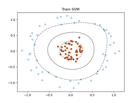
5. Train SVM
#---------------------------------------------------------------------------------------
# 3. Train SVM
#---------------------------------------------------------------------------------------

def plot_svc_decision_function(model,ax=None):
    if ax is None:
        ax = plt.gca()
    xlim = ax.get_xlim()
    ylim = ax.get_ylim()

    x = np.linspace(xlim[0],xlim[1],30)
    y = np.linspace(ylim[0],ylim[1],30)
    Y,X = np.meshgrid(y,x)
    xy = np.vstack([X.ravel(), Y.ravel()]).T
    P = model.decision_function(xy).reshape(X.shape)

    ax.contour(X, Y, P,colors="k",levels=[-1,0,1],alpha=0.5,linestyles=["--","-","--"])
    ax.set_xlim(xlim)
    ax.set_ylim(ylim)

X,y=make_circles(factor=0.2,noise=0.1) #factor = R2/R1, noise=std
clf = SVC(kernel="rbf").fit(X,y)
plt.scatter(X[:,0],X[:,1],c=y,s=30,cmap=plt.cm.Paired)
plot_svc_decision_function(clf)
plt.title('Train SVM')
plt.savefig('./img/RBFkernelSVM.png')
plt.show()
참고자료
https://scikit-learn.org/stable/modules/svm.html#classification
1.4. Support Vector Machines — scikit-learn 0.24.2 documentation
1.4. Support Vector Machines Support vector machines (SVMs) are a set of supervised learning methods used for classification, regression and outliers detection. The advantages of support vector machines are: Effective in high dimensional spaces. Still effe
scikit-learn.org
https://www.programmersought.com/article/84594638865/
SVM nonlinear simple implementation - Programmer Sought
Study notes for small crayons from sklearn.datasets import make_circles X,y = make_circles(100, factor=0.1, noise=.1) X.shape y.shape plt.scatter(X[:,0],X[:,1],c=y,s=50,cmap="rainbow") plt.show() clf = SVC(kernel = "linear").fit(X,y) plt.scatter(X[:,0],X[:
www.programmersought.com
https://jakevdp.github.io/PythonDataScienceHandbook/05.07-support-vector-machines.html
In-Depth: Support Vector Machines | Python Data Science Handbook
To handle this case, the SVM implementation has a bit of a fudge-factor which "softens" the margin: that is, it allows some of the points to creep into the margin if that allows a better fit. The hardness of the margin is controlled by a tuning parameter,
jakevdp.github.io
https://broscoding.tistory.com/145
머신러닝.make_circles 사용하기
import numpy as np import pandas as pd import matplotlib.pyplot as plt from sklearn.datasets import make_circles X,y=make_circles(factor=0.5,noise=0.1) # factor = R2/R1, noise= std) plt.scatter(X[:,..
broscoding.tistory.com
위키독스
온라인 책을 제작 공유하는 플랫폼 서비스
wikidocs.net
'공부 > 컴퓨터비젼' 카테고리의 다른 글
| [컴퓨터비전 과제] 7. CNN(Convolution Neural Network) (0) | 2021.06.10 |
|---|---|
| [컴퓨터비젼 과제] Epipolar Geometry (0) | 2021.05.14 |
| [컴퓨터비젼] 13. Stereo (0) | 2021.04.18 |
| [컴퓨터 비젼] 11.Single-View Modeling (0) | 2021.04.18 |
| [컴퓨터 비젼] SIFT(Scale Invariant Feature Transform (1) | 2021.04.12 |


